The Mathematical Heresy That Warmed the World: How Fourier’s Heat Equation Broke Calculus and Built the Modern Age

In the early 1800s, a French mathematician–physicist sat down with what looked like a purely practical problem:

How does heat flow through a solid body?

The answer he wrote down did not just found a new branch of physics. It declared war on the way mathematicians thought about functions, curves, and even what it means to “solve” an equation.

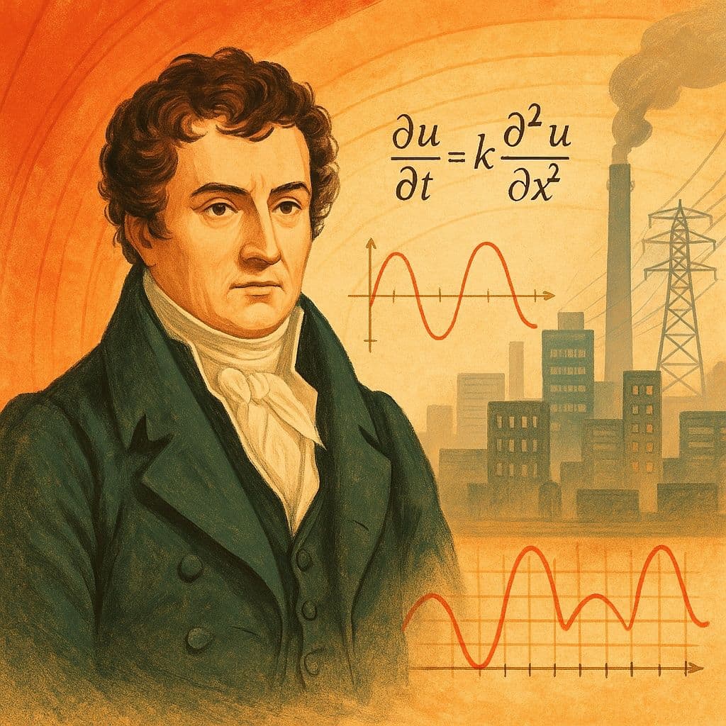
His name was Joseph Fourier, and his “heat equation” triggered one of the most profound conceptual shifts in mathematics. What began as a model for temperature in a metal bar ended up rewriting calculus, inventing modern signal processing, and, quite literally, helping us understand how the world warms and cools.

This post is about that heresy: why Fourier’s work looked wrong to his contemporaries, why it was (mostly) right, and how its echoes still shape every simulation, every image, every digital sound you experience today.

1. From Baking Bread to Partial Differential Equations

The physical idea Fourier had is simple enough:

• A solid body has a temperature field $u(x,t)$: temperature at point $x$ and time $t$.

• Heat flows from hotter to colder regions.

• The rate of change of temperature is governed by local curvature of the temperature profile.

For a long, thin, homogeneous rod, ignoring cross-section variation, the temperature $u(x,t)$ is essentially 1-D. Fourier argued (building on and clarifying earlier ideas) that it satisfies

$\frac{\partial u}{\partial t} = k \,\frac{\partial^2 u}{\partial x^2}$,

where:

• $u(x,t)$ = temperature,

• $x$ = spatial coordinate along the rod,

• $t$ = time,

• $k > 0$ = thermal diffusivity (a constant depending on material).

This is the heat equation.

At first glance, it looks like just another differential equation. But its solutions behave in a very distinctive way:

• They smooth out irregularities (sharp jumps blur over time).

• They propagate influence instantly (mathematically, any local heat disturbance immediately affects the whole rod, however slightly).

• They naturally bring in boundary conditions and initial conditions as part of the solution story.

The question Fourier attacked was:

Given the initial temperature $u(x,0) = f(x)$ on a rod, what is $u(x,t)$ for $t > 0$?

To answer this, he used a method that turned the rigorous analysts of his time absolutely furious.

2. The Classical Method: Separation of Variables

Let’s consider a simple setup.

• Rod of length $L$.

• Ends are kept at temperature $0^\circ$ (say, contact with ice baths): $u(0,t) = 0, \quad u(L,t) = 0 \quad \text{for all } t > 0$.

• Initial profile $u(x,0) = f(x)$ is given.

We seek $u(x,t)$ satisfying

$\frac{\partial u}{\partial t} = k\,\frac{\partial^2 u}{\partial x^2}, \quad 0 < x < L,\ t > 0$,

with the boundary and initial conditions above.

The standard trick in PDEs is separation of variables: we guess a special form

$u(x,t) = X(x) T(t)$,

where $X$ depends only on $x$ and $T$ only on $t$.

Substituting into the heat equation:

$\frac{\partial u}{\partial t} = X(x) T'(t), \quad \frac{\partial^2 u}{\partial x^2} = X''(x) T(t)$,

so

$X(x) T'(t) = k\, X''(x) T(t)$.

Assuming $X$ and $T$ are not identically zero, we can divide:

$\frac{T'(t)}{k\,T(t)} = \frac{X''(x)}{X(x)}$.

The left-hand side depends only on $t$, the right-hand side only on $x$; the only way this can be true for all $x$, $t$ is if both sides equal a constant, say -$\lambda$:

$\frac{T'(t)}{k\,T(t)} = \frac{X''(x)}{X(x)} = -\lambda$.

We get two ordinary differential equations:

$\begin{cases} T'(t) + \lambda k\, T(t) = 0, \\ X''(x) + \lambda\, X(x) = 0. \end{cases}$

The boundary conditions $u(0,t)=u(L,t)=0$ translate to

$X(0) = 0, \quad X(L) = 0$.

The spatial equation with these boundary conditions is a classic Sturm–Liouville problem. Solving:

• For $\lambda > 0$, we get oscillatory solutions.

• For $\lambda = 0$ or $\lambda < 0$ with these boundary conditions, only the trivial solution remains.

The nontrivial eigenfunctions occur for

$\lambda_n = \left(\frac{n\pi}{L}\right)^2, \quad n = 1,2,3,\ldots$,

with

$X_n(x) = \sin\left(\frac{n\pi x}{L}\right)$.

The corresponding temporal part:

$T_n(t) = e^{-k\lambda_n t} = e^{-k (n\pi/L)^2 t}$.

So each separated solution has the form

$u_n(x,t) = \sin\!\left(\frac{n\pi x}{L}\right) e^{-k (n\pi/L)^2 t}$.

Because the heat equation is linear, we can superpose:

$u(x,t) = \sum_{n=1}^{\infty} b_n \sin\!\left(\frac{n\pi x}{L}\right) e^{-k (n\pi/L)^2 t}$.

The coefficients $b_n$ must be chosen to match the initial condition $u(x,0)=f(x)$:

$f(x) = \sum_{n=1}^{\infty} b_n \sin\!\left(\frac{n\pi x}{L}\right)$.

And here is where Fourier’s heretical step truly begins.

3. Fourier’s Bold Claim: Every Reasonable Function Is a Trig Series

The equation

$f(x) = \sum_{n=1}^{\infty} b_n \sin\!\left(\frac{n\pi x}{L}\right)$

is not a differential equation; it’s a statement about representing an arbitrary function as an infinite series of sines.

Fourier went much further: he claimed that a huge class of functions-even those with corners, cusps, or discontinuities-could be written as (or at least approximated by) such series.

In its most famous form, a Fourier sine series on $(0,L)$ is

$f(x) \sim \sum_{n=1}^{\infty} b_n \sin\!\left(\frac{n\pi x}{L}\right)$,

with coefficients given by

$b_n = \frac{2}{L} \int_0^L f(x) \sin\!\left(\frac{n\pi x}{L}\right)\,dx$,

provided $f$ is “nice enough” (piecewise smooth, for example).

More generally, on $-\pi,\pi$ one writes a full Fourier series:

$f(x) \sim \frac{a_0}{2} + \sum_{n=1}^{\infty} \Big(a_n \cos(nx) + b_n \sin(nx)\Big)$,

with

$a_n = \frac{1}{\pi}\int_{-\pi}^{\pi} f(x)\cos(nx)\,dx,\qquad b_n = \frac{1}{\pi}\int_{-\pi}^{\pi} f(x)\sin(nx)\,dx$.

Today, most students see this as a standard tool in any intro PDE or signals course. But in Fourier’s time, this was shocking.

Why?

Because Fourier was happily writing expansions of functions that were:

• not differentiable at some points,

• sometimes discontinuous,

• not satisfying the conditions under which previous mathematicians felt safe using infinite series.

To his critics, it looked like he was saying:

“Take any function f. I don’t care if it has kinks, jumps, or worse. I’ll just chop it up into infinitely many sine and cosine waves, and we’re done.”

For mathematicians steeped in the idea that functions came from analytic expressions (finite compositions of algebraic operations, powers, roots, exponentials, etc.), this was basically heresy.

4. Why It Looked Like Heresy (and Kind of Was)

Before Fourier, infinite series were used, but mostly for functions that were already “nice”. For example, Taylor series expansions:

$e^x = \sum_{n=0}^{\infty} \frac{x^n}{n!}, \quad \sin x = \sum_{n=0}^{\infty} (-1)^n \frac{x^{2n+1}}{(2n+1)!}$,

and so on-smooth, analytic functions where the series come from repeated differentiation.

Fourier, by contrast, said:

“Give me a nasty function f. I won’t differentiate it millions of times. I’ll just integrate f against sines and cosines, and that infinite series is the function (in some sense).”

Two big problems offended the taste of his contemporaries:

Discontinuities and corners The functions coming from physics (e.g., initial temperature profiles) could be piecewise defined. Think of $f(x) = \begin{cases} 1, & 0 < x < L/2,\\ 0, & L/2 < x < L, \end{cases}$ a step-like profile. Fourier would still happily write a sine series for it. But how can a sum of smooth sines and cosines produce a function with a jump?

Convergence and meaning Mathematicians were not yet clear on:

• In what sense does a series converge to a function?

• Can we interchange limits, integrals, and sums freely?

• What happens at points of discontinuity?

Fourier’s arguments were often intuitively physical rather than strictly epsilonic. He had an engineer’s courage: if the series gives the right temperature as time evolves, and matches experiments, it must be okay.

His critics (including giants like Lagrange, Poisson, and Laplace) were uneasy. They sometimes used similar expansions themselves in private calculations, yet attacked Fourier’s bold general statements in public.

The result? A crisis of rigor-and, paradoxically, the birth of modern analysis.

5. The Heat Equation as an Infinite-Dimensional Low-Pass Filter

Let’s return to the solution formula we got from separation of variables:

$u(x,t) = \sum_{n=1}^{\infty} b_n \sin\!\left(\frac{n\pi x}{L}\right) e^{-k (n\pi/L)^2 t}$.

Notice what the time factors $e^{-k (n\pi/L)^2 t}$ do:

• For small n (low spatial frequencies), the exponent is small, so these modes decay slowly.

• For large n (high spatial frequencies: sharp corners, rapid oscillations), the exponent is large, so these modes decay quickly.

In more physical/mathematical language:

The heat equation acts as a low-pass filter on the initial data.

If your initial profile $f(x)$ is rough, with sharp edges, its Fourier sine series has many high-frequency components. As time progresses, those high-frequency components get exponentially damped, and the temperature profile becomes smoother and smoother.

After a long time, the solution essentially collapses to the dominant lowest modes:

$u(x,t) \approx b_1 \sin\!\left(\frac{\pi x}{L}\right) e^{-k (\pi/L)^2 t} \quad \text{for large } t$,

since all higher $n$ modes have decayed more strongly.

This is a key conceptual leap:

To understand the evolution of a system, decompose it into modes (sine/cosine waves), each with its own decay rate, then superpose.

This modal point of view is now standard everywhere:

• in vibrations and acoustics,

• in structural engineering,

• in quantum mechanics (energy eigenstates!),

• in climate and weather models.

But it started with Fourier’s heat equation and his willingness to break the then-current notion of what a function is.

6. How Fourier “Broke” Calculus-and How Others Rebuilt It

Fourier’s work forced mathematicians to confront uncomfortable questions:

What is a function, actually? Is it just something given by a single analytic formula? Or can it be given piecewise, or even arbitrarily on an interval?

When is a series representation valid? If $f(x) = \sum_{n=1}^{\infty} a_n \varphi_n(x)$, in what sense do we mean equality? Pointwise? Uniformly? In some integral average sense?

What kind of objects are sine series describing? Could there exist functions that are nowhere differentiable but arise as limits of smooth partial sums?

These puzzles motivated later giants:

• Dirichlet and Riemann clarified conditions for pointwise convergence of Fourier series.

• Weierstrass constructed continuous but nowhere differentiable functions-showing that the intuitive link between “curve” and “smoothness” is fragile.

• Lebesgue invented a new integral and measure theory to capture convergence and function spaces more precisely.

• Hilbert and others formalized function spaces (like what we now call $L^2$) where Fourier series converge in a precise sense.

In modern language, what Fourier was doing can be seen as expansion of $f$ in the orthonormal basis of functions

$\left\{ \sqrt{\frac{2}{L}} \sin\!\left(\frac{n\pi x}{L}\right) \right\}_{n=1}^{\infty}$

of the Hilbert space $L^2(0,L)$. The statement

$f(x) = \sum_{n=1}^{\infty} b_n \sin\!\left(\frac{n\pi x}{L}\right)$

then becomes, more carefully,

$\left\| f - \sum_{n=1}^N b_n \sin\!\left(\frac{n\pi x}{L}\right) \right\|_{L^2(0,L)} \to 0 \quad \text{as } N \to \infty.$

Fourier had none of that formalism-just physical intuition and integrals. In that sense, he “broke” the comfortable classical calculus built on smooth functions by forcing analysts to face the full wildness of function space.

7. From Iron Bars to the Internet: Why This Still Matters

Fourier’s heresy has quietly become the default mental model for almost everything continuous in the modern world.

7.1. Heat, diffusion, and climate

The heat equation is a prototype of diffusion equations. Replace temperature by concentration or probability, and you get models for:

• diffusion of pollutants,

• pricing in mathematical finance (Black–Scholes is essentially a heat equation in disguise),

• random walks and Brownian motion,

• and, in more complex forms, components of climate models.

Whenever we talk about how heat moves in soil, oceans, or the atmosphere, we are using descendants of Fourier’s equation. The idea that systems naturally decompose into modes with different decay rates underpins climate response functions, global circulation models, and the conceptual language of “fast” and “slow” processes in Earth’s energy balance.

7.2. Vibration, sound, and quantum states

Replace temperature by displacement or pressure, and Fourier’s modal thinking solves:

• vibrating strings → wave equation decomposed into normal modes,

• air columns in instruments → harmonics,

• quantum wavefunctions → expansions in eigenfunctions of the Hamiltonian.

The notion that a state can be decomposed as

$\psi(x) = \sum_n c_n \phi_n(x)$,

where $\phi_n$ are eigenfunctions with eigenvalues $E_n$, and time evolution just attaches phases $e^{-iE_n t/\hbar}$ to each mode, is directly analogous to how we decomposed $f(x)$ into sines and attached decays $e^{-k\lambda_n t}$.

The “mode thinking” is pure Fourier.

7.3. Digital signal processing and data compression

Your voice on a call, your music, your images, your videos-every one is touched by a discrete version of Fourier’s idea.

• The Fast Fourier Transform (FFT) computes discrete Fourier coefficients of a sampled signal: $x_k \approx \sum_{n=0}^{N-1} X_n e^{2\pi i nk/N}$.

• Audio formats like MP3, image formats like JPEG, and lots of video codecs rely on variants of Fourier-like transforms (cosine transforms, wavelets).

The core trick:

Take a complicated signal $x(t)$.

Decompose it into frequencies.

Throw away components too small to notice.

Store/transmit only the significant ones.

That’s Fourier series with attitude.

Every time you compress a photo, you’re relying on the same philosophy Fourier used on temperature:

Break the “shape” into basic harmonics; keep the important ones; you don’t need the rest.

8. The Heat Equation as a Metaphor for Understanding

There’s also a philosophical angle I like: the heat equation models forgetfulness.

Let’s write the solution again:

$u(x,t) = \sum_{n=1}^{\infty} b_n \sin\!\left(\frac{n\pi x}{L}\right) e^{-k (n\pi/L)^2 t}$.

• High-frequency details (sharp spikes, noise) vanish quickly: large n means fast decay.

• Low-frequency structure (broad shape) persists: small n decays slowly.

This is not only a thermometer story; it’s a metaphor for information:

• Systems dominated by diffusion “forget” microscopic structure and remember only large-scale patterns.

• Data pipelines that smooth and average effectively apply a heat-equation-like operation.

Mathematically, applying the heat semigroup $e^{t k \frac{d^2}{dx^2}}$ to a function $f$ is like convolving $f$ with a Gaussian kernel. In fact, on the real line, the fundamental solution is

$u(x,t) = \frac{1}{\sqrt{4\pi k t}} \int_{-\infty}^{\infty} \exp\!\left( -\,\frac{(x-y)^2}{4kt} \right) f(y)\,dy$.

The Gaussian kernel

$G_t(x-y) = \frac{1}{\sqrt{4\pi k t}} \exp\!\left( -\,\frac{(x-y)^2}{4kt} \right)$

spreads and smooths. This expression is, in a sense, just another way to say:

We decomposed into Fourier modes, damped each by $e^{-k\lambda_n t}$, and reassembled.

Two different viewpoints-Fourier series and Gaussian convolution-are mathematically equivalent for the heat equation. That equivalence is one of the crown jewels of analysis, and it grew out of Fourier’s “illegitimate” expansions.

9. The Price of Heresy: Gibbs Phenomenon and the Edge of Convergence

Of course, Fourier’s ideas weren’t perfect. One of the strange things you see when expanding a discontinuous $f$ into its Fourier series is the Gibbs phenomenon:

• Near a jump discontinuity, the partial sums of the Fourier series overshoot the height of the jump by about 9%, and this overshoot does not vanish as you take more and more terms-it just gets narrower.

Concretely, consider the $2\pi$-periodic square wave

$f(x) = \begin{cases} 1, & 0 < x < \pi,\\ -1, & -\pi < x < 0, \end{cases}$

extended periodically. Its Fourier series is

$f(x) \sim \frac{4}{\pi}\sum_{n=0}^{\infty} \frac{1}{2n+1} \sin\big((2n+1)x\big)$,

a pure sine series over odd harmonics. The partial sums wiggle and overshoot at the discontinuities. The more terms you add, the narrower the wiggle, but the peak overshoot amplitude tends to a fixed fraction of the jump height.

This phenomenon perfectly illustrates both the power and subtlety of Fourier’s expansions:

• The series is “right” in a global, integrated, or $L^2$ sense.

• But pointwise behavior, especially at “bad” points, can be surprising.

It took decades of work after Fourier to sort out all these subtleties. Yet, from the viewpoint of heat flow, Fourier was effectively right: the physical rod never has a perfect step-it always gets smoothed a bit, and the Fourier approach gives precisely the smoothed profile you measure.

10. Conclusion: The Heresy That Became the Canon

Fourier started with a down-to-earth question: how does temperature evolve in a solid? To answer it, he:

Wrote down a partial differential equation—the heat equation—that captures diffusion.

Solved it by decomposing the initial condition into sine and cosine modes.

Asserted that “essentially any” reasonable function can be represented by such a trigonometric series.

At the time, this looked like a radical departure from the “safe” world of smooth, analytic functions. His contemporaries saw gaps, hand-waving, even contradictions. But the physical predictions worked. The math community was forced to respond-not by rejecting his ideas, but by reinventing analysis:

• defining functions more broadly,

• understanding convergence more subtly,

• building function spaces (like $L^2$),

• and developing a theory where Fourier’s expansions make rigorous sense.

The payoff?

• Heat transfer and diffusion theory,

• signal processing and compression,

• vibration and quantum mechanics,

• probability and stochastic processes,

• climate and energy balance modeling.

All of these are, in spirit, descendants of Fourier’s “heresy”.

So the next time you see a Fourier series

$f(x) = \frac{a_0}{2} + \sum_{n=1}^{\infty} \big(a_n \cos(nx) + b_n \sin(nx)\big)$,

or solve a heat equation

$\frac{\partial u}{\partial t} = k \,\frac{\partial^2 u}{\partial x^2}$,

remember: you are not just doing a textbook exercise. You are touching a piece of mathematical rebellion that reshaped our understanding of functions, phenomena, and, in a very literal sense, how the world warms and cools.

If you’d like, I can help you:

• shorten this into a LinkedIn-style summary post about Fourier and modern modeling,

• or cut it into mini-sections for an Instagram/Telegram series with one formula and one “wow-fact” per post.